| NA3 | Volker Freudenthaler |  |
| |||||||
|
Test of the optical
setup with partial telescope cover
Goal:
- test and verify the
alignment of laser and optics and Principle: - determine the distance of full overlap. - compare lidar signals
from different parts of the telescope
aperture. Additional tests: - far range: Rayleigh calibration
("matching method") - near range (overlap): multi-angle (elevation) measurements 1
Introduction
2 Update after L'Aquila workshop Oct. 2007 => nomenclature 3 Presentation of results and calculation of deviations 1 Introduction In a perfect lidar system the backscattered rays from all lidar ranges within the measurement range have the same transmission in the optical system. In the near range the total transmission decreases, because some rays are vignietted by the field-of-view aperture and/or other apertures, which results in the overlap function. At the same time rays with large incident angles in the telescope - and therefore with large incident angles on interference filters etc. - can have reduced transmission due to the angular wavelength shift with incident angle of the interference filters. - overlap - vignetting - angular effects We can use this behaviour to check the performance and alignment of the optical system, because the ray-bundles from different parts of the telescope aperture travel through the optical setup in different paths (see figure 1) and with different incident angles on the optical elements (see figure 2b). 
Figure 1: ZEMAX model of the MULIS lidar
system. Rays from different parts of the telescope have different paths
through the optical system. Shown are rays from telescope cover sections
"TopIn" and "BottomOut" as explained below. 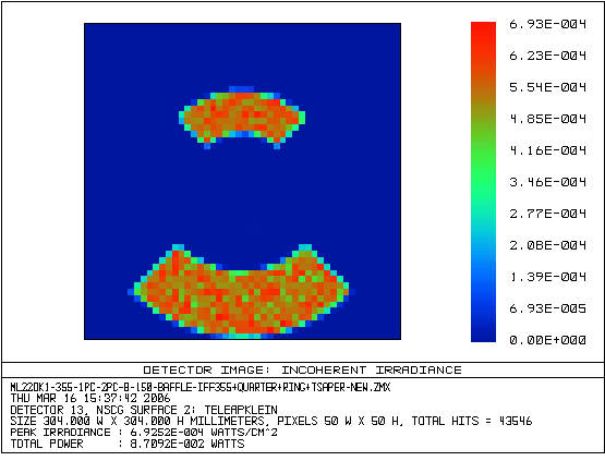 (2a)
(2a) 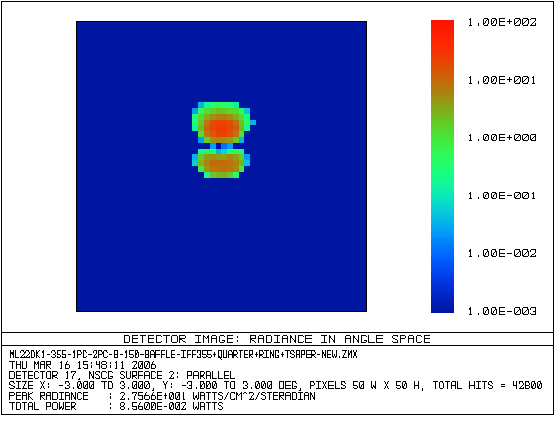 (2b)
(2b)Figure 2a and b: Rays from different parts
of the telescope (left picture shows intensities in the telescope aperture
like fig.1) have different ray angles in the collimated beam after the
collimation lens (right picture). The blue square in the right picture has
a total width and height of 6°. In the upper spot are the ray angles of
the "TopIn" section of the telescope, and in the lower spot are the angles
of the "BottomOut" section. This shows that the rays from "BottomOut" are
about 1° more inclined after the collimation lens than the
"TopIn"-rays.The example is a simulation of the Munich MULIS lidar system
for rays backscattered from 150 m lidar range. In other words: when we compare the range dependend lidar signals of rays-bundles from different parts of the telescope aperture we can find the differences in the transmission losses due to vignietting and due to the angular dependend transmission of the different ray paths . We can do this by covering the telescope aperture with opaque cardboard for example and subsequently measuring only ray-bundles from one of the eight or four sections shown in figure 3a. Eight sections give more information and the differences are more pronounced, but four sections are faster to measure and are probaly sufficient for a fast check. The "Top" section is oriented from the telescope optical axis towards the laser optical axis as shown in figures 3b and 3c. "Left" and "Right" are with respect to viewing towards the telescope. 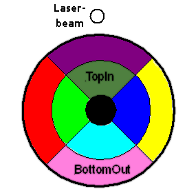 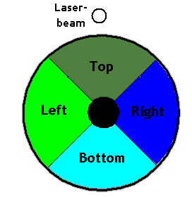 (3a) (3a)
 (3b) (3b)
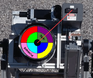 (3c) (3c)
Figure 3: Proposed test sections of
the covered telescope aperture (3a) and orientation with respect to the
telescope-laser axes (3b and 3c). For convenience I use the abbriviations TI, LI, BI, RI, TO, LO, BO and RO for TopIn, LeftIn .... BottomOut and RightOut, respectively, in the following. A ZEMAX simulation of such measurements for the 607 nm channel of the MULIS with a otpimized telescope and without interference filter is shown in figure 4. The range step of the calculations is 25 m. The MULIS telescope (see fig.1) has a diameter of 300 mm, a focal length of 960 mm, and in this cases a fov diaphragm with 3.6 mm diameter, which results in about +-2 mrad fov. The laser beam diameter is 8 mm with 0.6 mrad fwhm divergence, the distance of the laser to the telecope axis is 400 mm, and the laser is pointing parallel to the telescope axis. We see in figure 4 that the TO-sector has full overlap close to 200 m but the BO-sector only from about 400 m on. Therefor the whole telescope has full overlap only further than 400 m range. 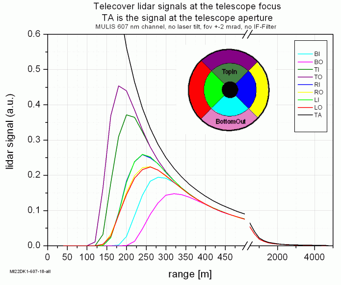 Figure 4: Zemax simulation of the 607 nm
channel signal (including optical transmission) of MULIS with an optimized
telescope using different telescope setions as indicated in the legend,
paralell pointing laser, and a fov of +- 2mrad. Note the change in range
scale above 500 m range. This can be seen much better if we plot the
signals relative to the calculated signal in the telescope aperture (TA,
black in fig. 4), which is displayed in figure 5. Here we see the
attenuation due to the aluminium coatings, and second that the full
overlap is actually reached later than 400 m. For the ZEMAX simulations I
will use this display. For our experimental signals we don't have the
calculated signal in the telescope aperture, and therefor we can use the
TO-sector as reference, which is shown in figure 6. 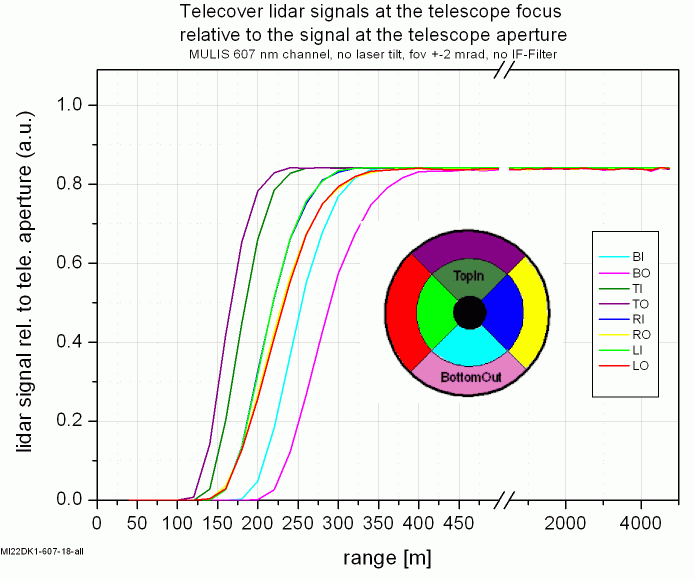 Figure 5: As figure 4 but signals reltive
to the calculated signal in the telescope aperture. 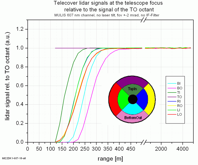 Figure 6: As figure 4 but signals relative to the signal of the TO-sector. Using only a single measurement with the full telescope we were not able to discern the influence of the always present boundary layer aerosol from the transmission effects of the optics. Comparing the eight measurements, which should be done with stable boundary layer conditions - best at night, we can not only determine the distance of full overlap, but by comparing them with a raytracing simulation we can also get hints about which part of the lidar is misaligned. 2 Update after L'Aquila workshop Oct. 2007: - Change of nomencalture (N-E-W-S,or
NO-NI-EO-EI-SO-SI-WO-WI, looking from the sky into the telescope). This
nomenclature seems to be more intuitive and introduces more options like
NW).


 Figure 7.: - In case all apertures
have the same effective area, the relative values of the signals can be
readily related to get information about the relative transmission of each
sector.
- Performing an addtional measurement after the procedure with the first sector used gives information about the order of atmopsheric changes during the measurements. - With monoaxial lidar configurations, the quarter and octant tests give mainly information about a possible laser tilt, and to a lesser extend about the overlap and angle dependend transmission of the optical system. Information about the latter can be achieved with "In-Out" tests, maybe with different ring diameters. Please inform me about your experiences with that. - For the publication of the EARLINET QA results we need a common layout - especially for the normalisation of the measurements. I proposed already to
A measured example using the range-calibration can be seen in figure 8.  Figure 8: NEWS (old: Top,Right,Bottom,Left) measurement example with one of the EARLINET systems using the range-calibration. In this case the relative differences between the two wavelengths show, that the NEWS differences are not due to atmospherical changes during the measurements. From my experience and ZEMAX simulations I guess that the NEWS differences are mainly due to the spatial inhomogeneity of the sensitivity of the used HAMAMATSU R7400 PMT (see Discovering detector inhomogeneities). 3 Presentation of results and calculation of deviations Proposal 1
- normalisation
I propose to use the range-calibration (explained above in chapter 2) for the presentation in the EARLINET-ASOS report, because - it can be applied in all situations, - noise/distortion in one profile does not influence the other profiles. Proposal 2 - range of data display I further propose to show the profiles up to 5 km in order to inlcude the normalisation and far range. With a coordinate break at an appropriate range both the near range (overlap, near range effects) and the far range (loss of signal due to laser tilt or else) can be displayed. If you can't do that and if a single plot doesn't show the near range clear enough, please present two plots, one for the near range and one for the whole range up to 5 km. Proposal 3 - calculation of deviations For the deviations I propose to calculate point by point
Proposal 4 - deviation limits Limits: I propose that if following limits are exceeded, the lidar system should be inspected and improved, and the deviations should be decreased below these limits:
=> Please comment on these proposals. In case of no replies I consider them as accepted for the first round of telecover checks. => Discussion on the next workshop. Telecover checkup and plot requirements The measurements should be sufficiently smoothed over range or time in order to keep the deviations due to signal noise well below the limits. The resolution of the plots should be large enough to show enough detail. The plots must contain information about
Monoaxial systems: In order to check laser tilt and other deviations, at least a quadrant and an In-Out test should be performed. An example for the above mentioned procedure is shown in figures 9 to 12 for the MULIS 532 nm channels, parallel (fig. 9 and 10) and perpendicular (fig. 11 and 12). In this case we can see, that the N-sector profile exhibits a relatively increased signal below about 2.5 km range. But actually there is a loss of signal in the far range due to a bad primary mirror with a lot of distortion in the north sector, which probably causes vignetting of its beam due to the field of view diaphragm similar in all channels. As a result, we don't use this sector for lidar measurements, and consequently we don't use it for the caclulation of deviations below. At long sight we will buy a new telescope. The comparison between the measurements E and E2 with the east sector at different times shows, that the atmosphere didn't change considerably during the measurements, and that the small cloud at 1.2 km didn't disturb too much. According to the limits in proposal 4, the full overlap of the parallel channel is at 320 m range, and the perpendicular channel should be inspected in order to reduce the RMS deviations AllDev below 0.1.  Fig. 9
  Fig.
10 Fig.
10 Fig.
11 Fig.
11 Fig.
12 Fig.
12Updated 18.09.06, 11.11.07 Volker Freudenthaler |